Seismic tomography allows the reconstruction of an image of the subsoil distribution of seismic wave velocity and its anomalies with high resolving power. In detail, refraction seismic survey is an indirect, active seismic survey that uses refracted waves generated by contrasts of waves velocity to reconstruct subsurface characteristics. The velocity of seismic waves depends on the density and elastic properties of the material crossed, i.e., properties attributable to the lithological characteristics of the substrate investigated. The direction of propagation of the waves in depth follows Snell’s law and at each interface there are phenomena of refraction, reflection and diffraction. In refraction surveys, as the name implies, only refracted waves will be considered. Refraction seismic tomography allows to obtain a picture of the velocity distribution in the subsurface highlighting the continuous changes in velocity rather than a layered model typical of refraction surveys ( Intercept, delaytime, plus minus, GRM).
The refraction seismic survey consists of generating a seismic wave of compression or shear (energization) and recording its arrival at the geophones arranged in a line at known intervals. The interpretation of the recorded measures is based on the analysis of the time taken by the wave generated with the energizations to reach each geophone. In order to reconstruct the speed variation of compression waves in the subsurface, it is necessary to perform several energizations in different positions along the line.
The measurements made using the refraction method can be processed using the tomographic procedure in order to highlight the local velocity variations in detail.
The tomographic technique involves the creation of an initial synthetic model of the subsurface and its perturbation in search of the minimum deviation between the measurements made on the ground and the “virtual” measurements recorded on the synthetic model through an iterative procedure that cycles between the following two phases:
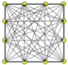
- In the ” forward ” phase, the arrival times of the seismic pulse are calculated on the synthetic model (smartTomo is based on the work of Moser, T. J. “Shortest path calculation of seismic rays.” Geophysics 56.1 (1991): 59-67). The initial velocity model is divided into a grid whose cells have assigned initial velocity values. On the sides of the cell are multiple nodes (the number of which is chosen by the user) that constitute the nodes of the network of hypothetical seismic rays that connect all sources and all receivers that are also themselves nodes. Each node is connected with nodes in neighboring cells. Increasing the number of nodes increases the detail and accuracy in the seismic ray path but also increases the memory usage. The path of the refracted wave corresponds to the path that takes the shortest time to travel between the source and the receiver.
In the “inverse” phase, the synthetic times calculated in the ” forward” step are compared with the times measured on the seismograms; the differences between the times are used to update the synthetic model (smartTomo employs an algorithm that can be traced back to the “Simultaneous Iterative Reconstruction Technique” family). In the implementation of this method the speed is replaced by its inverse, the slowness. For example, considering a generic seismic radius j between the source and the receiver the average slowness can be expressed as:
(1) 
where tij is the measured time between the source (i-th) and the receiver (j-th) and lij is the length of the j-th sisimic ray. Therefore, knowing the measured path times tm and the calculated path time tc for the j-th ray, the residual path time can be calculated:
(2) 
The residual of the path times is projected onto each cell k on which the slowness correction factor is also calculated as:
(3) 
The index i represents each seismic ray incident on the k-th cell. The slowness correction factor will be used to update the velocity model at the end of each iteration of the resolution cycle. This procedure yields a model, with continuous velocity variations and not necessarily constrained by the presence of strong refractors like the bedrock.
Each update cycle is followed by a smoothing phase of the result in order to make the model more homogeneous by means of velocity distribution operations to the cells adjacent to those crossed by the seismic beams; this process ensures greater stability to the calculation procedures and a more easily interpretable result.
The procedure is illustrated in Figure 2 from Reinhard Kirsch, “Groundwater Geophysics – A Tool for Hydrogeology” Springer 2006.
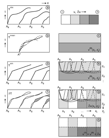
Image summarizing seismic tomography processing.
(a) Dromochrone measured on the traces recorded on the ground are used to build the initial model (b) and (c).
(d) Using the initial model, (e) synthetic dromochrone are calculated.
(f) Differences between measured and simulated dromochrone are calculated (equation 2) and updates to the velocity model (g) are calculated (equation 3)
(h) The updated velocity model can be used as a new initial model in (d) and (e) until a specified stop criterion has been reached