The dromochrone or travel-time curves are plots in which the arrival times of seismic waves are represented as a function of distance from the source. They find their use in localizing the position of earthquakes, in reflection and refraction seismic surveys. In this post we will address their use in refraction seismic and how they are also useful in traveltime-based refraction seismic tomography.
The dromochrone graph is a diagram in which one axis reports the position of the receivers (or the distance from the source) and on the other axis is indicated the time taken to reach the receivers by a given type of seismic wave.
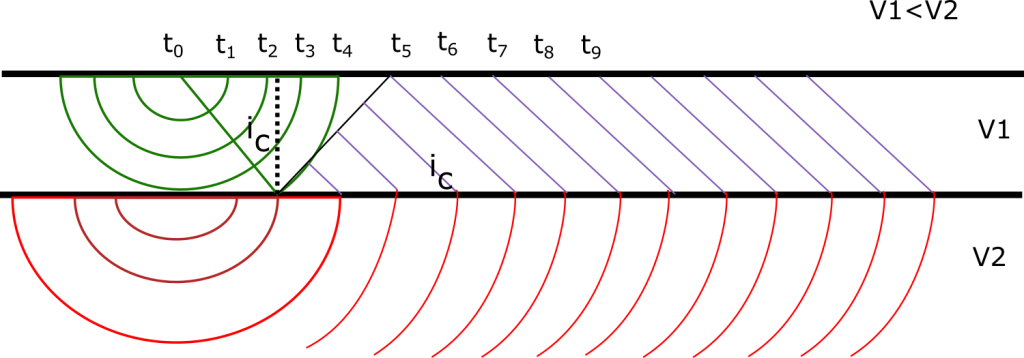
The seismic waves when they meet materials characterized by different velocities give origin to refraction and reflection phenomena. When they hit an interface characterized by increasing speed with depth (V2 > V1) with an angle equal to arcsin(V1/V2) called critical angle, the waves travel parallel to the interface and for the principle of Hyugens part of the energy returns to the surface giving rise to the head waves, represented in purple in the diagram above. Measuring the arrival time of the waves at different distances and representing them on a graph we obtain the following plot.
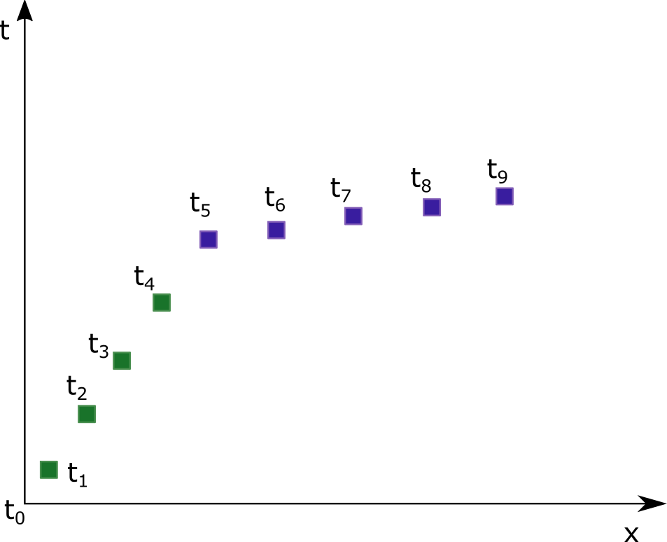
In a model with two uniform horizontal layers where the underlying layer has a velocity V2 > V1 the dromochrone graph is represented by two straight segments. The graph is represented on the plane defined by the distance and time axes so the inverse of the slope of the segment represents the apparent velocity of the crossed layers, i.e.:
(1) 
Where X is the position between the receivers or between a receiver and the source while time T is the time required to reach the receivers.
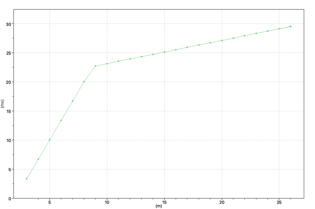
For example, in the image below, the first layer identified by the arrivals between an X equal to 3 and an X equal to 9 corresponding to arrival times of about 3 ms and 23 ms. The speed of the first layer will consequently be
(2) 
After the X = 9 coordinate, the dromochrone changes slope and indicates that the waves generating the first arrivals have encountered a faster layer and have undergone refraction at a critical angle.
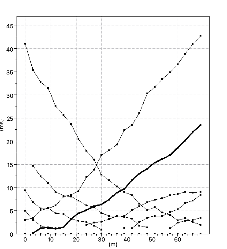
For the interpretation of refraction seismic with the intercept time technique it is necessary to determine the slope of the dromochrone, the crossover point and the intercept time. On the contrary, for tomographic processing only the travel time is important but, of course, refraction must be present, i.e. increasing the distance from the energization position must change the dromochrone slope indicating an increase in velocity. The dromochrone, as in the case of the following image, will be more flattened at greater distances.
Situations in which the dromochrone breakpoint does not occur, i.e., does not contain a refraction, cannot be interpreted with refraction tomography. The break point may occur with a sharp inflection point or in a softer manner, but must be present. A sharp break may indicate a well-defined interface (e.g., the soil cover placed on the bedrock), while a softer dromochrone break will show a progressive increase in velocity with depth.
The following image, represents dromocores that do not show the correct bending (break point), indicating instead an increase in arrival times with increasing distance.
This dromochrone arrangement does not fit the interpretation with the refraction technique. Using SmartTomo the resulting profile would often be just a row of cells whose velocity would try to optimize arrival times through direct waves only.
This situation should be identified already in the field during the survey to understand if it could be due to acquisition problems (e.g., poorly evident first arrivals) or to actual characteristics of the site and therefore the need to perform different type of surveys.