smartTomo 2027.0: boreholes come into the program, meet MjolNET

Anyone who does refraction tomography knows the scene. It is evening, the spread has ninety traces, there are twelve shots to pick and the model has not even started yet.

Version 2027.0 starts from that scene. We worked on every step, from the comparison with boreholes to the drawing that lands on the client’s desk. In the middle is MjolNET, our artificial intelligence system.
Boreholes are inside smartTomo

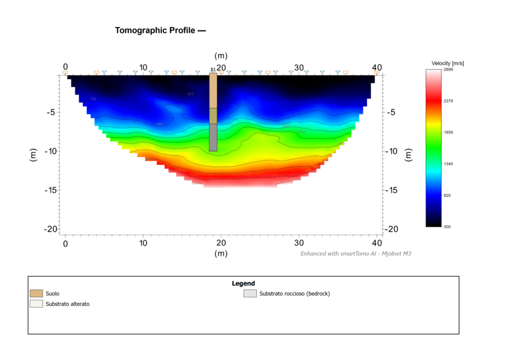
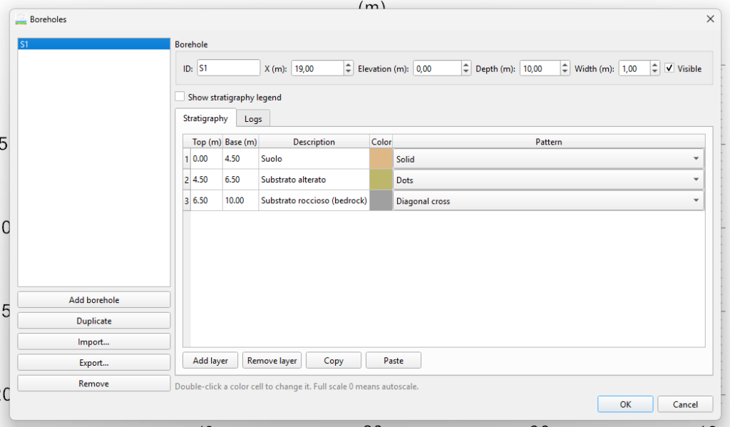
A velocity section is only really understood next to a borehole. Until now that comparison happened outside smartTomo, by hand. In 2027.0 boreholes are imported from CSV, XLSX, ODS and AGS4 and drawn on the section, with their stratigraphic legend. They also appear in the refraction processing window, over the profile.

If a file contains an error, for example a base above its own top, the program flags it in the list. Data can be exported to CSV and AGS4.
Loading Boreholes on the section, with stratigraphic legend.

MjolNET: artificial intelligence that helps, not replaces

MjolNET is the artificial intelligence system of smartTomo. It was built for one purpose: to help the person who interprets, not to take their place. The decisions stay with you. MjolNET proposes, shows and compares.

MjolNET is private. It does not collect data and does not transmit any.

In 2027.0 MjolNET has two networks, M1 and M3. They are optional: if you do not turn them on, smartTomo works as before.

MjolNET M1: the picker that knows when to stop

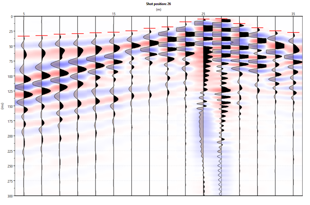
M1 reads the traces and proposes the first arrivals. Nothing strange so far, automatic pickers have existed for a long time. The difference is this: M1 knows when not to trust itself.

If a trace is too noisy, M1 does not invent a pick. It leaves the trace free and the picking stays with you. Automatic work covers the clear traces and your attention goes where it is needed.

Energy-ratio picking is still in the program. You can use either, or compare them on the same spread.

MjolNET M3: a second look at the model

Every inverted model deserves a critical eye. Is that velocity contrast a structure or an artefact? M3 is the second look. It works on the model you have already inverted and produces a filtered version.

You decide whether to use it. With AI Difference Map you see at once where M3 acted and by how much. With AI Filter Comparison you put the two models side by side. Every image that comes from the filter carries an “AI” watermark, so nobody mistakes the filtered model for the original.
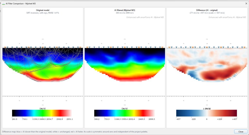
Original model, model filtered by MjolNET M3 and difference map.

How M1 and M3 work is explained in the white paper.

The drawing is composed inside smartTomo

The last step used to be the dullest: export the images and reassemble them elsewhere. The new Print layout editor composes the drawing directly in the program. It has multiple pages, rulers, title block, legend, time-distance curves, colour bar and spread geometry.

A drawing that works can be saved as a template and reused on the next project. Export produces PDF, PNG, SVG, Word and OpenDocument.
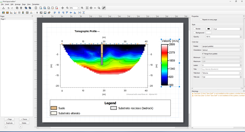
A sheet composed in the Print layout editor.

Small things you notice every day

  • Metres or feet, your choice, for distances, axes and annotations.
  • Horizontal or vertical colour bar, with adjustable fonts.
  • A preview of every palette in the menu.
  • A floating magnifier for manual picking.
  • JSON export with geographic coordinates and EPSG code.

Under the hood the computation is faster, the model uses less memory and parallelism is more stable.
Link

Brochure

User guide

smartTomo 2025.0 released

We are pleased to announce the release of SmartTomo 2025.0 ‘Punta Marguareis’! This new version represents a major step forward in the development of seismic refraction tomography, introducing seismic attenuation tomography.

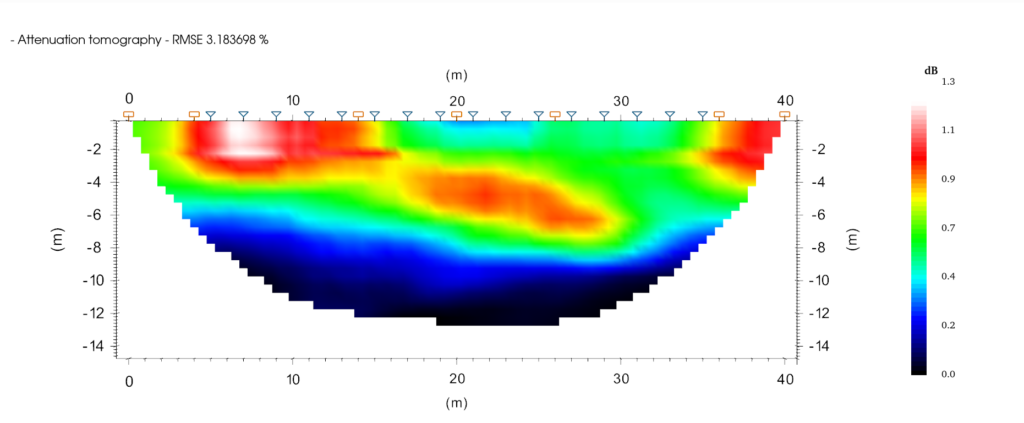
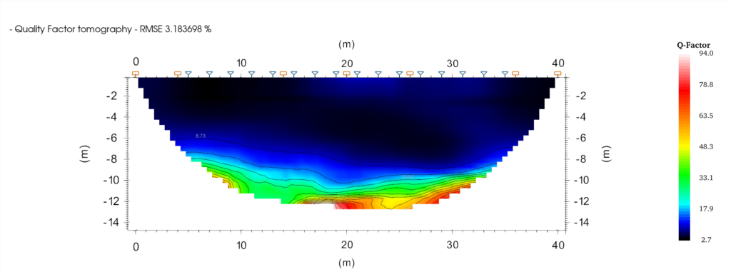
Attenuation and Q-Factor tomography

The latest version introduces a significant step forward in seismic refraction tomography processing by including seismic attenuation tomography.

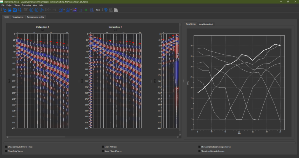
This new processing enables seismic attenuation and Q-Factor tomography by analysing how the energy of the refracted signal attenuates along the profile. The signal intensity is sampled within a defined window around the first arrival, which can be selected manually track by track.

This type of analysis is complementary to traditional seismic wave velocity tomography and provides additional information on subsurface properties. However, for the results to be reliable, it is essential to avoid the introduction of artificial and variable attenuation factors, such as unevenly installed geophones (some set in the ground, others placed on rigid surfaces such as asphalt) or different gains between acquisition channels.

New visualisation of seismic traces

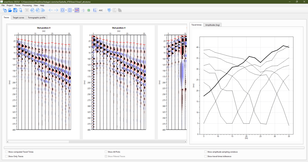
Seismic traces can now be displayed together with the signal intensity map to better highlight waveforms.

Editing dei tempi di arrivo

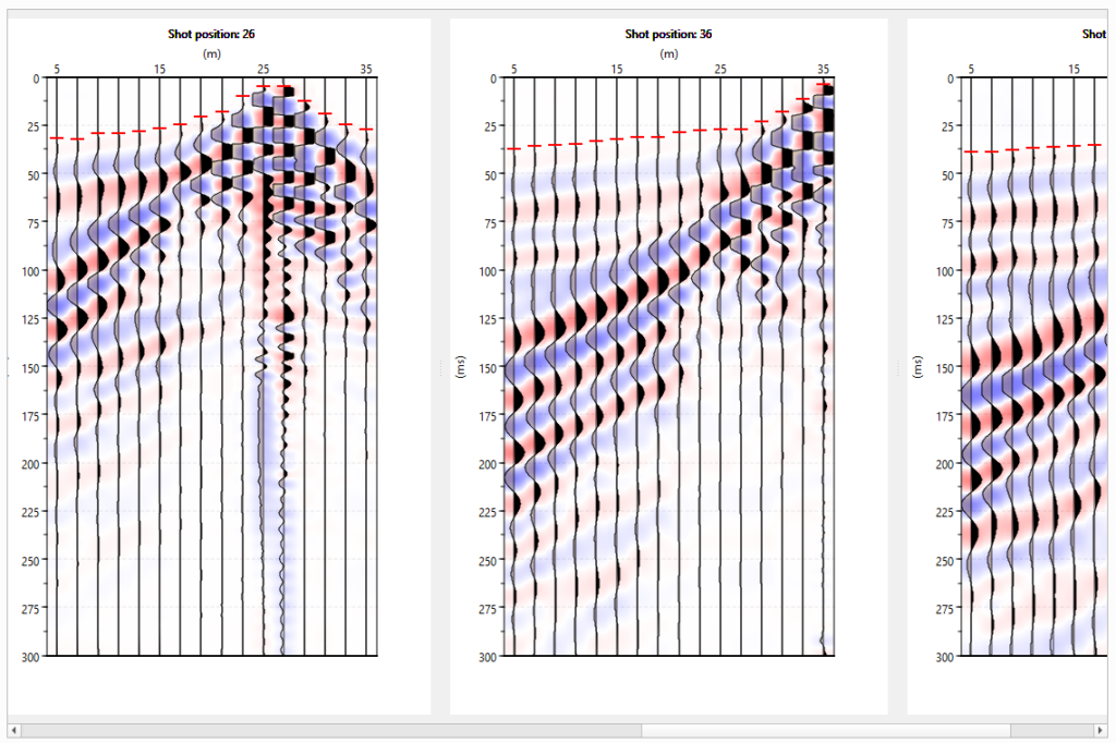
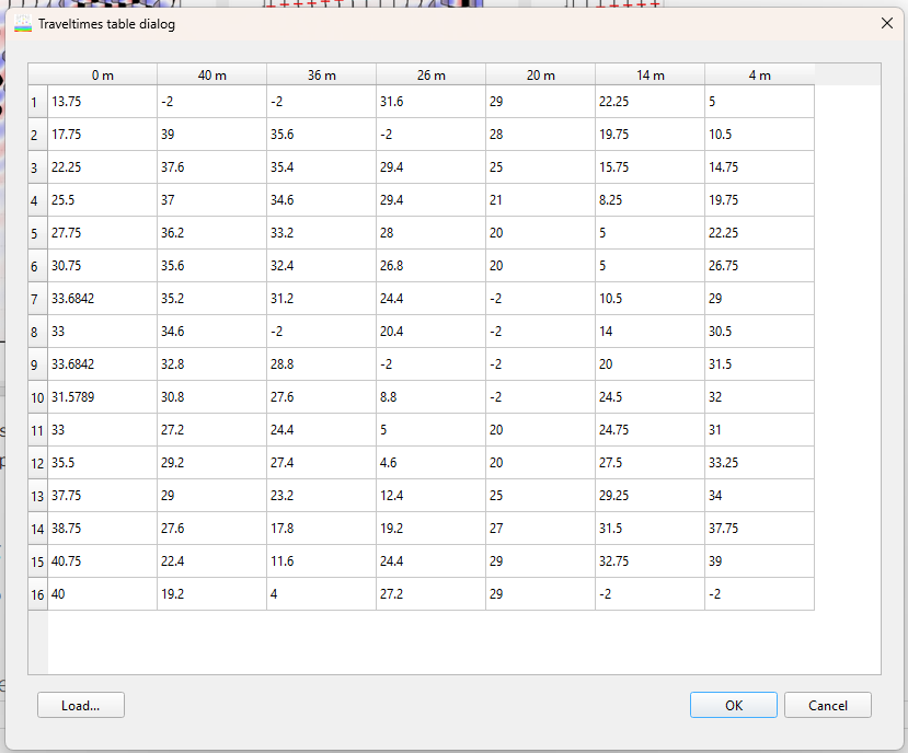
From this version, it is possible to display, copy and paste first-arrival times into a table showing measured values expressed in milliseconds. This function then allows the first arrival times to be edited manually for more accurate identification.

Smoothing parameter

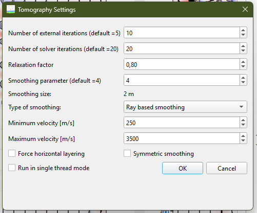
The smoothing parameter, previously expressed in number of cells, is now converted to its equivalent in metres. This update provides a more intuitive and immediate indication of the effect of smoothing on the profile, making it easier to adjust the parameter according to the size of the area under investigation and improving the interpretation of results.

Dark/light themes

Now smartTomo can be run in light or dark mode or be automatically set to match the style of the desktop.

Undo last processing

This version introduce the undoing of the last tomography processing allowing user goes back to the previous tomographic model.

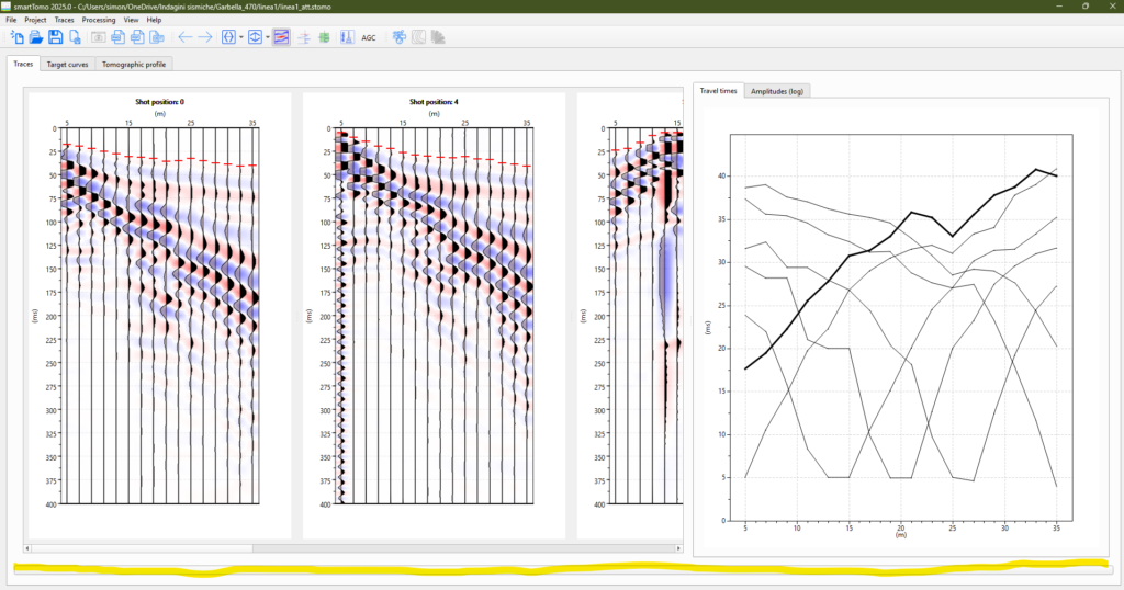
Hide/show the bottom tool widget

Further updates

Since the fix5 update of this release, smartTomo allows you to export the tomography directly to Surfer’s GRD format. This allows you to view the results in Surfer without having to convert them from the text table

Release notes of SmartTomo 2022.0

Spalshscreen of smartTomo

We are happy to announce the release of the new version of SmartTomo, the best version to date.
The new version includes improvements in seismic tomography processing, profile visualization, and new result export options, in addition to the inevitable bugfixes.

Seismic tomography processing

This image has an empty alt attribute; its file name is immagine-1024x702.png

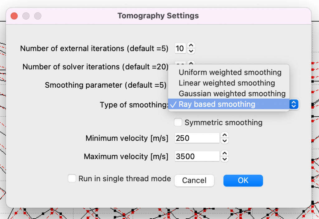
A new seismic ray-based smoothing mode has been added. This new smoothing method uses only the velocity value of the cells crossed by the seismic rays. The velocity distribution function follows a law based on the speed of the seismic waves giving more continuity where the speed is higher. This smoothing allows for more velocity variation in the superficial layers and a relatively smoother profile at deeper depths.

Profile visualization

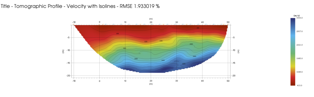
Seismic Profile with Grid and Title - SmartTomo 2022
Seismic Profile with Grid and Title – SmartTomo 2022

The profile visualization module has received several improvements.
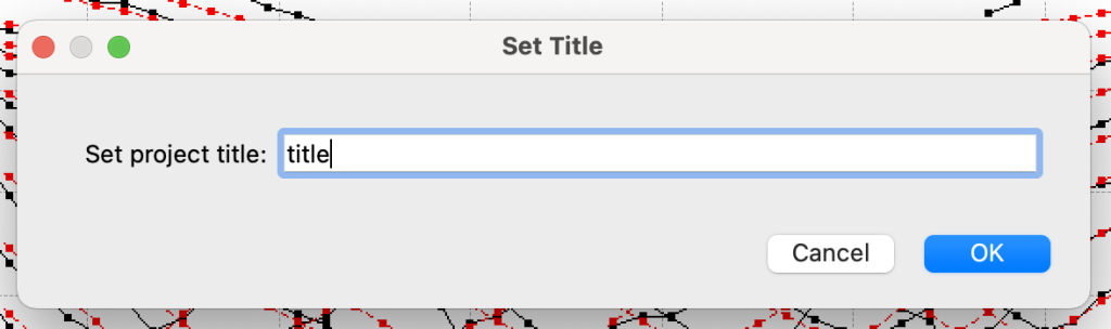
It is now possible to assign a title to the profile that will be displayed at the top of the view. In addition to the name, the view type and the RMSE error of the simulation are shown. The title and RMSE error will be saved in the project so that they can be recalled when opening the project again.

Dialog to set the title in smartTomo
Set the title

The profile can now be displayed also with a grid overlay corresponding to the major intervals shown on the axes.

Information Density Level Viewer

This image has an empty alt attribute; its file name is immagine-1-1024x396.png
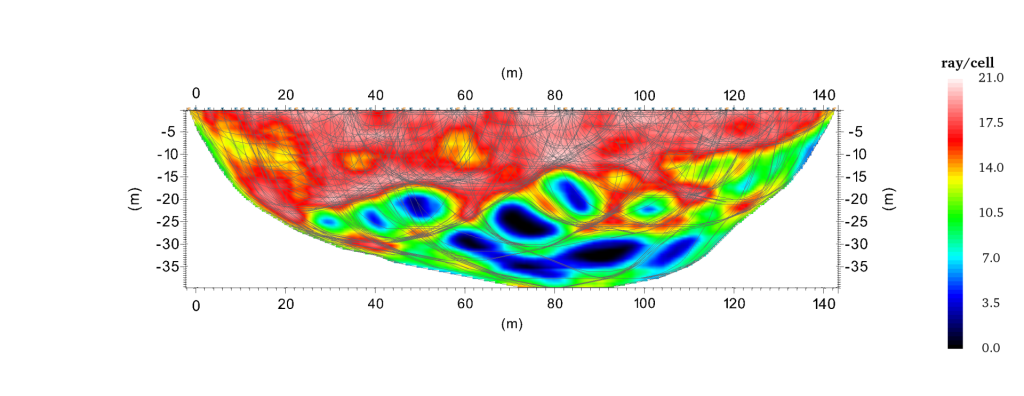
View of the Information Density Level

In SmartTomo 2022 a new way of displaying the results has been added: the information density layer. This layer is intended to represent how much each individual cell was affected during model reconstruction. Higher values correspond to cells whose value has been determined by a larger number of measured data (equations) always taking into account that the tomographic inversion process is an optimization of the model and not an exact solution.
This visualization then allows you to assess whether the tomographic model in a given area has been updated and with how many constraints.

Export of results

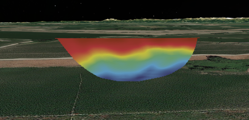
Seismic profile exported in KML and shown in Google Earth
Profile exported to KML and displayed in Google Earth

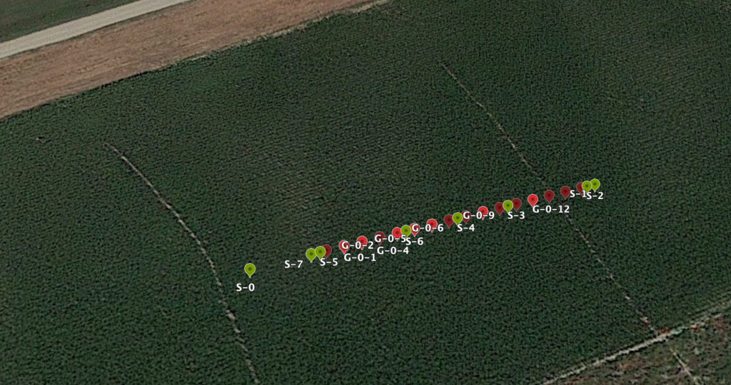
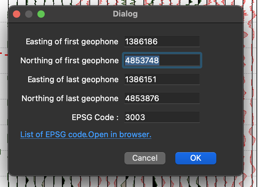
SmartTomo 2022 introduces the possibility to export results in KML format for visualization in external tools such as Google Earth. For the export it is necessary that the seismic profile is georeferenced (first and last geophone) and that the coordinate system EPSG code is defined.

This image has an empty alt attribute; its file name is Schermata-2021-11-24-alle-17.50.26-1024x540.png
Geopositioning and energization exported in KML and visualized in Google Earth
This image has an empty alt attribute; its file name is Schermata-2021-11-02-alle-19.10.58.png
Setting of coordinates in a projected reference system like UTM