Anyone who does refraction tomography knows the scene. It is evening, the spread has ninety traces, there are twelve shots to pick and the model has not even started yet.
Version 2027.0 starts from that scene. We worked on every step, from the comparison with boreholes to the drawing that lands on the client’s desk. In the middle is MjolNET, our artificial intelligence system.
Boreholes are inside smartTomo
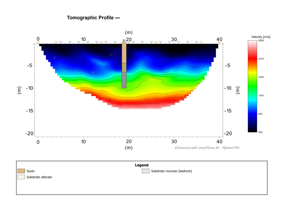
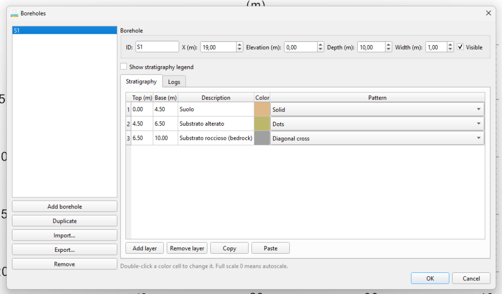
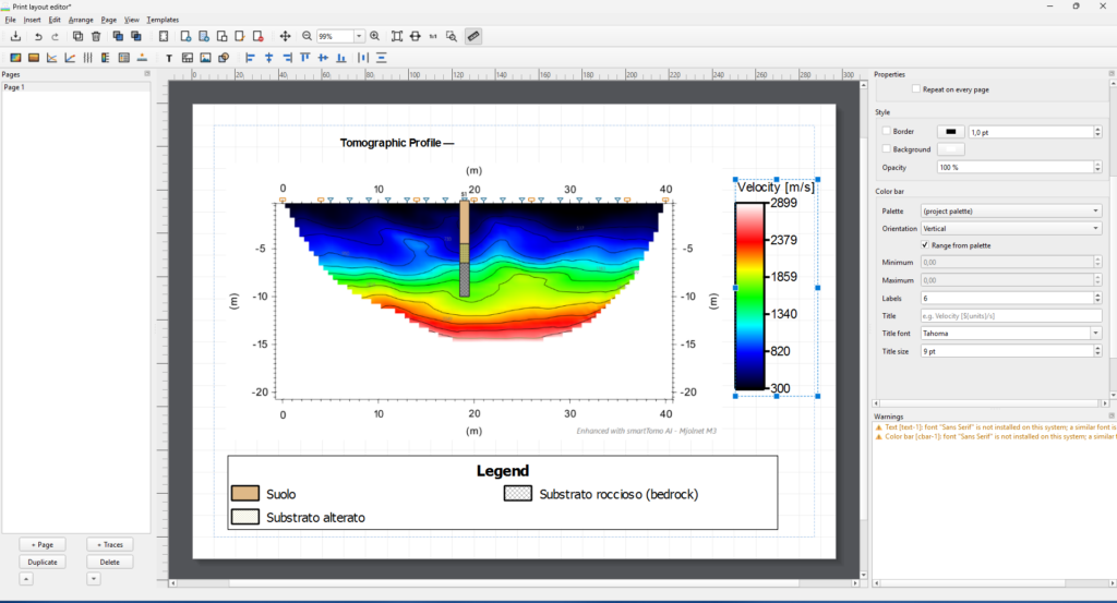
A velocity section is only really understood next to a borehole. Until now that comparison happened outside smartTomo, by hand. In 2027.0 boreholes are imported from CSV, XLSX, ODS and AGS4 and drawn on the section, with their stratigraphic legend. They also appear in the refraction processing window, over the profile.
If a file contains an error, for example a base above its own top, the program flags it in the list. Data can be exported to CSV and AGS4.
MjolNET: artificial intelligence that helps, not replaces
MjolNET is the artificial intelligence system of smartTomo. It was built for one purpose: to help the person who interprets, not to take their place. The decisions stay with you. MjolNET proposes, shows and compares.
MjolNET is private. It does not collect data and does not transmit any.
In 2027.0 MjolNET has two networks, M1 and M3. They are optional: if you do not turn them on, smartTomo works as before.
MjolNET M1: the picker that knows when to stop
M1 reads the traces and proposes the first arrivals. Nothing strange so far, automatic pickers have existed for a long time. The difference is this: M1 knows when not to trust itself.
If a trace is too noisy, M1 does not invent a pick. It leaves the trace free and the picking stays with you. Automatic work covers the clear traces and your attention goes where it is needed.
Energy-ratio picking is still in the program. You can use either, or compare them on the same spread.
MjolNET M3: a second look at the model
Every inverted model deserves a critical eye. Is that velocity contrast a structure or an artefact? M3 is the second look. It works on the model you have already inverted and produces a filtered version.
You decide whether to use it. With AI Difference Map you see at once where M3 acted and by how much. With AI Filter Comparison you put the two models side by side. Every image that comes from the filter carries an “AI” watermark, so nobody mistakes the filtered model for the original.
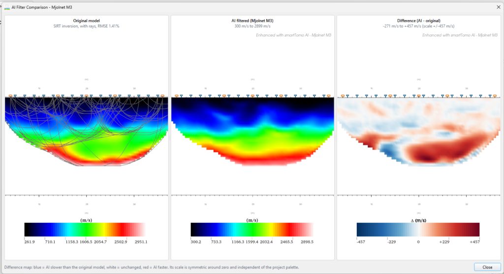
How M1 and M3 work is explained in the white paper.
The drawing is composed inside smartTomo
The last step used to be the dullest: export the images and reassemble them elsewhere. The new Print layout editor composes the drawing directly in the program. It has multiple pages, rulers, title block, legend, time-distance curves, colour bar and spread geometry.
A drawing that works can be saved as a template and reused on the next project. Export produces PDF, PNG, SVG, Word and OpenDocument.
Small things you notice every day
- Metres or feet, your choice, for distances, axes and annotations.
- Horizontal or vertical colour bar, with adjustable fonts.
- A preview of every palette in the menu.
- A floating magnifier for manual picking.
- JSON export with geographic coordinates and EPSG code.
Under the hood the computation is faster, the model uses less memory and parallelism is more stable.